Y How Much Will Gdp Change If Firms Increase Their Investment By $8 Billion And The Mpc Is 0.80?

The Aggregate Expenditures Model

Section 01: The Aggregate Expenditures Model

Now we will build on your understanding of Consumption and Investment to form what is called the Aggregate Expenditures Model. This model is used equally a framework for determining equilibrium output, or Gross domestic product, in the economy. When nosotros developed the Consumption Part in a previous lesson, we stated that Consumption was a function of Disposable Income. In this model, we return to the assumption of the Circular Menstruation Model that the production of the final goods and services in the economy (the GDP) results in a menstruum of income that is exactly equal to the value of that output. Since the GDP is equal to Income, we tin model the Spending (for now just Consumption and Investment) in the economy in terms of GDP instead of in terms of Income.

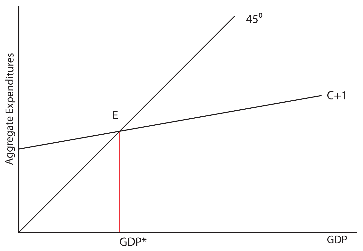
In the above graph, nosotros labeled point Eastward every bit the equilibrium point and Gross domestic product* as the equilibrium level of the Gdp. Allow'southward explore why Due east is equilibrium. Remember that i of the characteristics of equilibrium is that if you move away from it, natural market forces should automatically movement you back toward the equilibrium. Observe this procedure in the graph below:

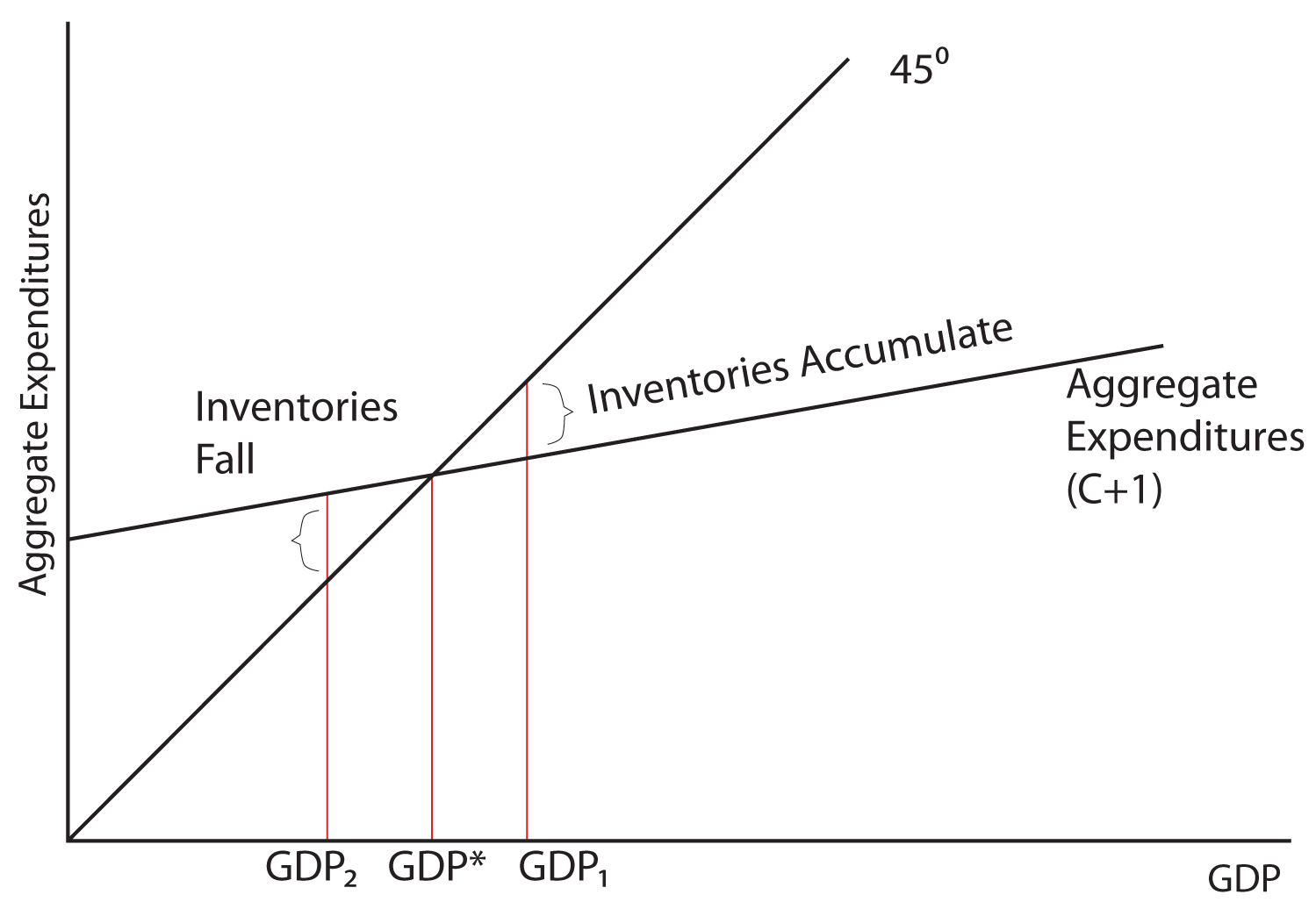
If the economy were for some reason producing at GDP1 instead of Gross domestic product*, what would be the consequence and what market forces might induce the economy to return to Gross domestic product*? Notice: at GDP1, total spending is less than output. We know that spending is less than output because at this level of Gdp the Aggregate Expenditures line is below the 45 degree line, which is the line where spending is equal to output. And then spending would be equal to output at point A, but actual spending as measured by the Aggregate Expenditures line is beneath that (labeled B). Imagine you are running the economy. Each month, you are producing ten,000 units of output and people are ownership 9,000 units of output. Each month, yous would exist calculation ane,000 units of output to your inventories and over the course of the year, inventories would be piling up. Imagine that producers have a sure level of inventories that they desire to have on hand, but that they do non desire the stock of inventories to substantially abound or depleted. At GDP1, inventories would be piling up at the rate of 1,000 actress units of inventory each calendar month! What would yous practise if y'all were running the economic system and unwanted inventories were building upwards? Wouldn't that be a signal to you to reduce production? Every bit you reduce product, output or the GDP, falls from GDP1 to GDP*.

What if the economy were producing at GDP2? Now the Aggregate Expenditure line is to a higher place the 45 degree line, indicating that spending is above output. Spending would be equal to output at point D, just bodily spending is at betoken F. Imagine that the economy is producing 5,000 units of output each month, but that consumers and businesses together are purchasing 6,000 units of output. How would it exist possible for more than to be bought than what is produced in any given time period? Information technology would be possible if businesses have unsold inventories on hand. But if a business has an ideal level for their inventories that they desire to maintain, and purchases exceed production, inventories will be drawn downwardly or depleted. What would naturally happen in an economy if spending were greater than production and inventories were falling? Businesses would brainstorm to produce more, and the output or Gross domestic product of the economic system would rise from GDP2 to Gdp*.

To summarize, notice that in this model:

1. If spending is greater than production, inventories will exist depleted and production will rise, and
2. If spending is less than production, inventories will accumulate and production will fall, And so ...
3. Equilibrium is achieved where production exactly equals spending:

Output = Spending

4. Or, in other words,

GDP = Consumption + Investment

GDP* is the equilibrium output of the economy because it is where output (GDP) is equal to spending (consumption + investment).

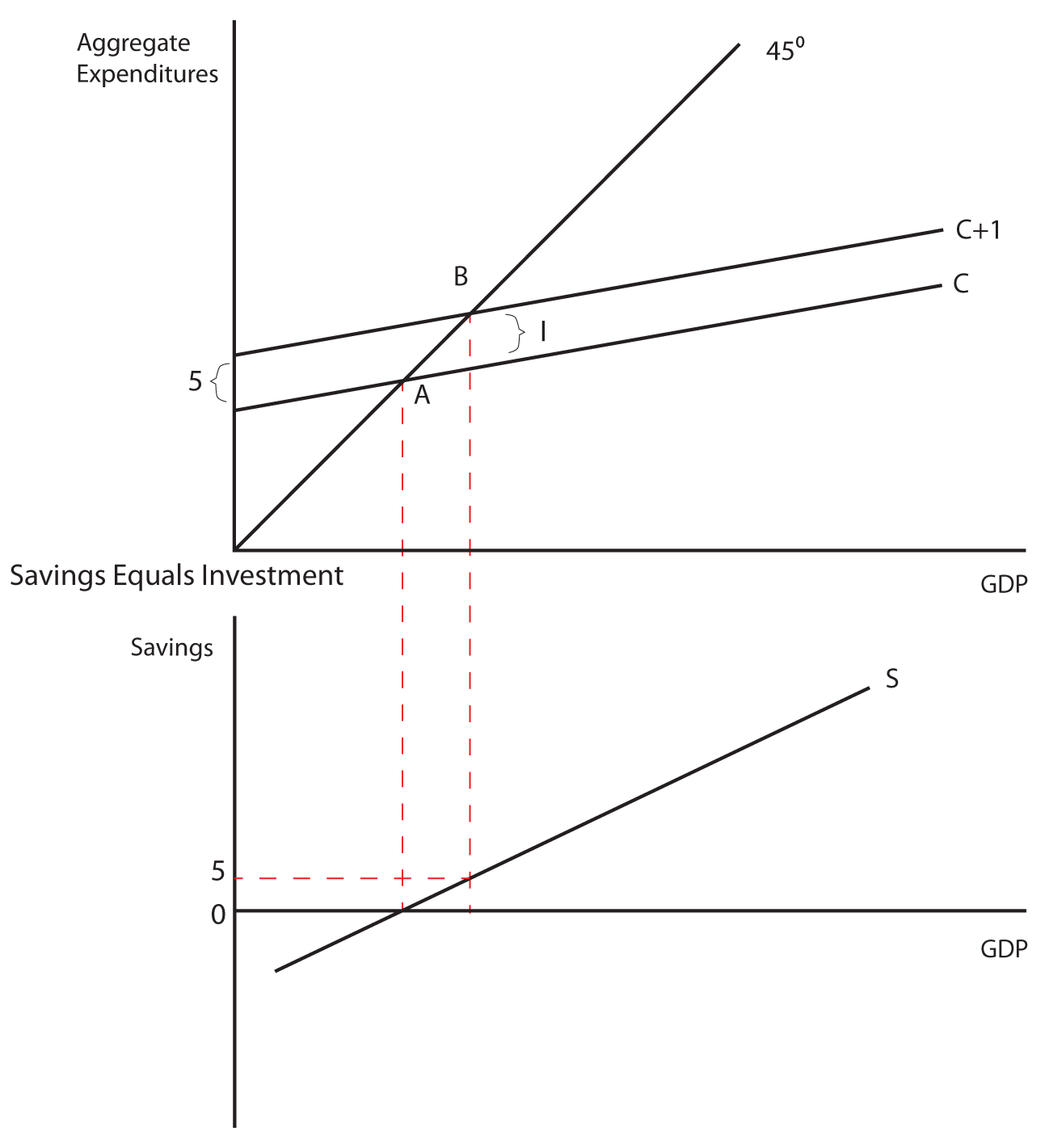
Savings and Investment

A 2d way of looking at equilibrium is through savings and investment. Remember that when people salve, they are withdrawing spending from the flow of income and expenditures. Savings is therefore chosen a leakage. When businesses invest, they are calculation spending to the menstruation of income and expenditures and so that Investment is chosen an injection.

Equilibrium output is accomplished when:

Leakages = Injections

or

Savings = Investment

If savings is greater than investment, then GDP is too high and output will fall. If savings is less than investment, then GDP is too depression and output will rise. Let'southward look at this graphically.

Retrieve About Information technology: Aggregate Expenditures

In the tabular array below is data for a hypothetical individual-closed economy. Private means that in that location is no regime and closed means that there is no foreign merchandise. We will consider a mixed (both a private and a authorities sector) and open (one that accounts for foreign merchandise) economy later. Use the data in this table to graph the amass expenditures line on one graph and the savings and investment schedules on some other graph. Prove how these graphs illustrate that the aggregate expenditures of the company are in equilibrium. This means "spending equals output" is the same thing as "savings equals investment."

Table 1: Equilibrium Example

Real GDP	Consumption	Savings	Investment	AE = C + I
xi,800	12,000	(200)	600	12,600
12,600	12,600	0	600	13,200
thirteen,400	13,200	200	600	13,800
fourteen,200	13,800	400	600	14,400
fifteen,000	14,400	600	600	fifteen,000
fifteen,800	15,000	800	600	15,600
16,600	15,600	1,000	600	xvi,200

The Investment Multiplier

The model of Aggregate Expenditures that we are currently considering is often called a Keynesian Model considering information technology was first formulated past British economist John Maynard Keynes in his General Theory of Employment, Interest, and Money, published in 1936—at the height of the nifty depression. One of the central premises of Keynesian economics is the idea of a multiplier. Keynes hypothesized that a given increase in spending would cause output to increase past a multiple of the increment in spending. How is this possible?

Permit's start with the case of Investment spending. When a business organisation spends $1 on new plant or equipment information technology injects $i into the economy. That $1 becomes income to someone (whoever built the machine or constructed the new plant) who spends a portion of it and saves the rest. The portion they spend and the portion they save depends on their MPC and their MPS. The portion that is spent becomes income to someone else who likewise spends a portion, which becomes income to another, who spends a portion, and so on. The spending stream can be characterized in the following fashion:

$ane + $1(MPC) + $ane(MPC)(MPC) + $1(MPC)(MPC)(MPC) + …

Or

$ane + $1(MPC) + $1(MPC)2 + $ane(MPC)3 + …

Which can be shown in its limit to equal 1/(1-MPC). This is called the Investment Multiplier. As long as the MPC is less than i, the multiplier volition be greater than one. In fact, we tin show that

1. When the MPC is .nine, the multiplier is x
2. When the MPC is .8, the multiplier is 5
3. When the MPC is .75, the multiplier is 4
4. When the MPC is .six, the multiplier is ii.5
5. When the MPC is .five, the multiplier is 2

Information technology should also exist stated that the investment multiplier can be shown in terms of the MPS. It is the reciprocal of the MPS, 1/MPS, since the MPS is equal to 1-MPC.

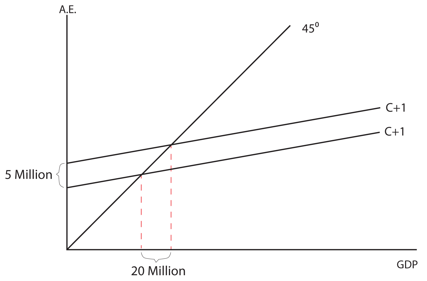
Example

Let's consider a scenario where firms in the economy decide to increase investment spending by five million dollars. If the MPC is equal to .75, the Investment Multiplier is equal to 4 and output in the economy will go upwardly by xx 1000000 dollars (the five million dollar increment in Investment times the multiplier of four). Graphically this is shown beneath:

Recall About It: Investment Multiplier Calculations

Based on the graphs given, answer the following questions.

1. In the first graph, if the MPC is 0.75, what is the new level of GDP when aggregate expenditures go up by two meg?

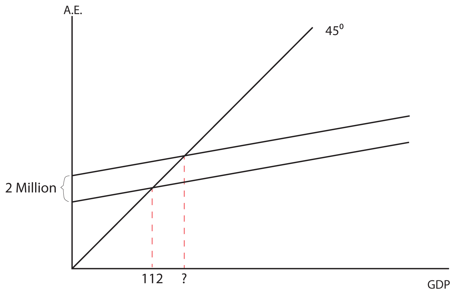
Respond

two. In this graph, what is the multiplier and what is the MPS?

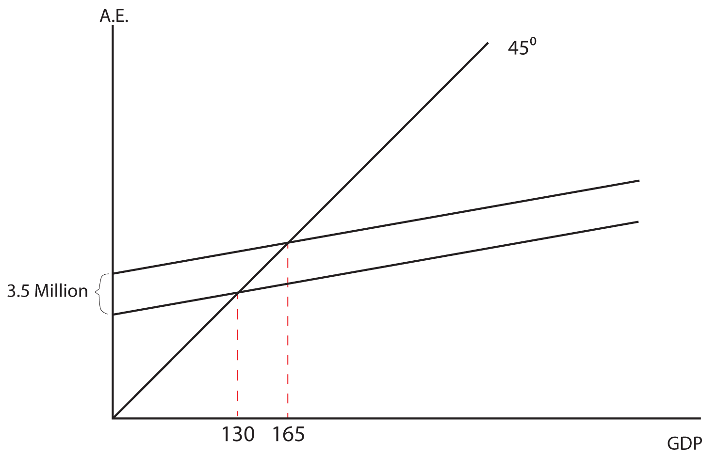
Respond

three. In this graph, if the MPS is 0.2, how much did aggregate expenditure go up by to get the indicated increase in GDP?

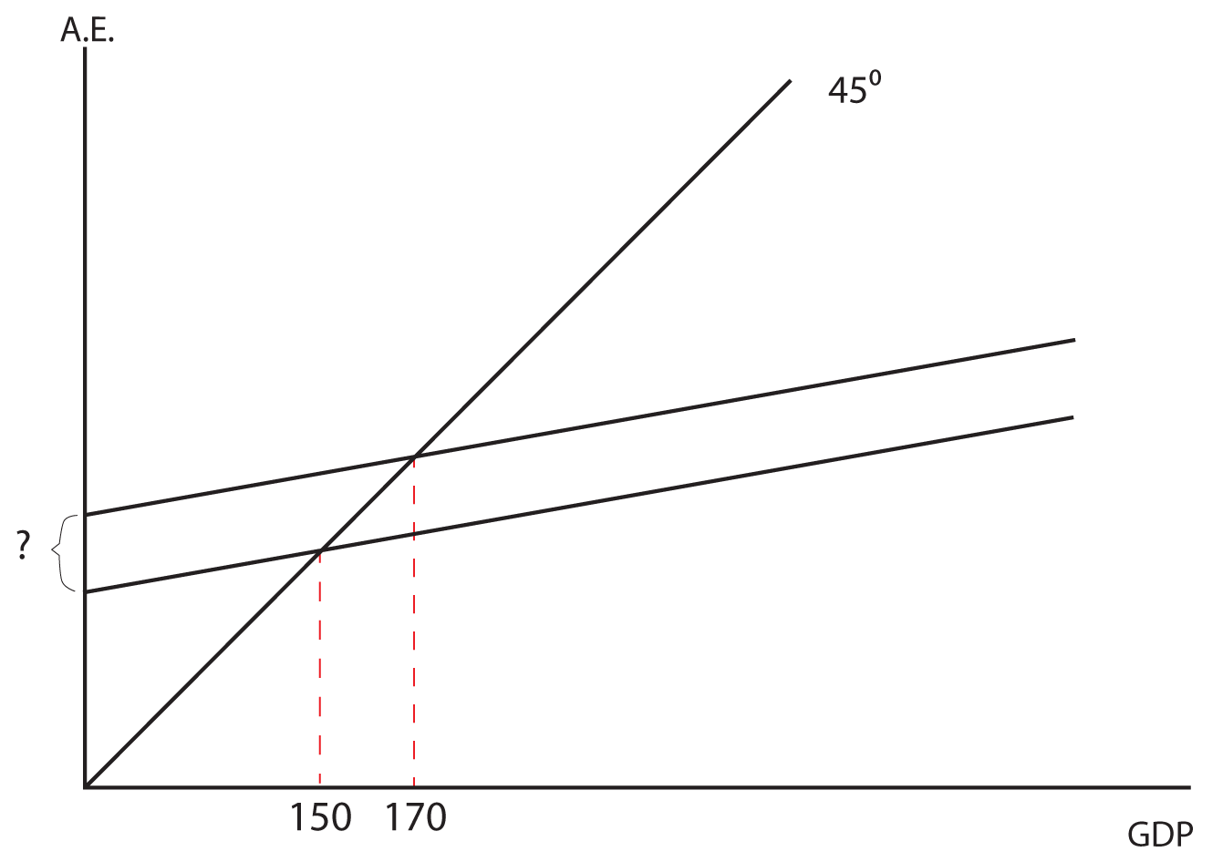
Reply

Department 02: Government Spending

Now let united states consider a mixed (both government and private spending) closed (no net exports) economy. The basic change is that we are now adding government spending to the model. Since government spending is determined by a political process and is not based on the level of the Gross domestic product, it is graphed every bit a horizontal line when Gross domestic product is on the horizontal centrality. When this horizontal line is added to the upward sloping Aggregate Expenditures line, it but shifts Aggregate Expenditure upward by the amount of the authorities spending. Meet the two graphs below for an illustration. The equilibrium Gross domestic product volition be determined by where the C+I+G line intersects the 45 degree line in our standard model.

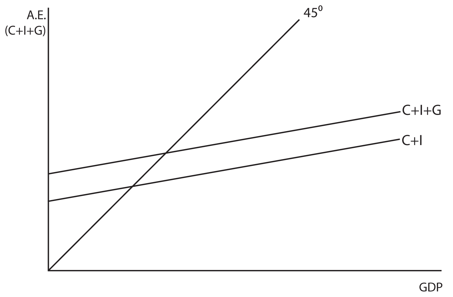
Changes in government spending have a similar impact on equilibrium GDP as changes in investment.

The Regime Spending Multiplier

Quantitatively, the government spending multiplier is the same as the investment multiplier. A $1 increase in government spending volition result in an increase in Gdp equal to $one times i/(1-MPC). Since the investment and government spending multipliers are the same, they are sometimes but jointly referred to as expenditure multipliers.

Recall About It: The Effects of Government Spending

This instance will illustrate the bear on Keynes felt a change in government spending would have on output in the economy. Assume that the MPC is equal to 0.half dozen. What does the regime spending multiplier equal? What bear on would a $5 billion increase in government spending have on equilibrium Gross domestic product? What about a $5 billion decrease in G? Can you illustrate both cases with a graph?

Reply

When the MPC is 0.6, the multiplier is two.5. The $v Billion change in One thousand will change the Gross domestic product by $12.v Billion if the MPC = 0.6. Shut (X)

The Tax Multiplier

Equally mentioned before, the spending multipliers are all the same, one/(i-MPC). There is too a multiplier that is associated with a change in taxes. Information technology is called the tax multiplier, and it is NOT the same as the spending multipliers. In fact, it is smaller than the spending multipliers. Why would the taxation multiplier exist smaller than the government spending multiplier? The reply lies in the fact that when a business or the government undertakes new spending, they inject the initial corporeality of that spending into the income stream and then it multiples through the economic system. When the regime decides to lower taxes, they are not injecting new coin into the economy; they are simply deciding not to accept money out of the economy that was already in the income stream. Individuals will then spend some portion of the money that they get to keep. Then, if the regime increases spending past $1 billion, the entire $i billion is injected into the income stream. If they reduce taxes past $ane billion, only the MPC x $1 billion is injected into the income stream. Therefore, the affect of the tax multiplier is:

$ane(MPC) + $1(MPC)(MPC) + $1(MPC)(MPC)(MPC) + …

This progression can exist shown to be equal to the spending multiplier times the MPC, or

MPC 10 1/(1-MPC)

Which is simplified equally

MPC/(1-MPC)

Since reducing taxes increases income and vice versa, the tax multiplier is negative, i.e.

-MPC/(1-MPC)

Allow's wait at some common values of the MPC and determine the tax multiplier for each.

1. When the MPC is .9, the revenue enhancement multiplier is -9
2. When the MPC is .viii, the tax multiplier is -4
3. When the MPC is .75, the tax multiplier is -3
4. When the MPC is .six, the tax multiplier is -1.5
5. When the MPC is .v, the tax multiplier is -1

Do you see the relationship between the expenditures multipliers and the taxation multiplier at each level of the MPC? How would yous draw it?

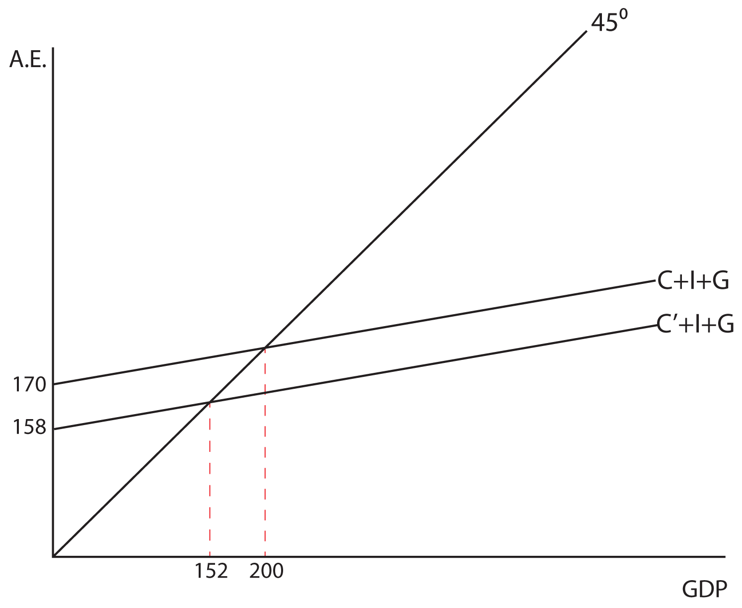
Note that a change in taxes shifts C in our aggregate expenditures model. An increase in taxes shifts C downward and a subtract in taxes shifts C upward with the expected impacts on equilibrium GDP.

Think About It: Product Possibilities

Bear witness how a modify in taxes has a specified touch on Gross domestic product, depending on the MPC. Show that you can get the aforementioned answer on its touch on GDP, using the tax multiplier or the expenditures multiplier. For example, let's say the authorities increases taxes by $16 Billion with an MPC = 0.75. What impact would this have on equilibrium GDP?

ANSWER

The direct respond involves using the tax multiplier. $16 billion x -iii = a $48 billion subtract in the Gross domestic product.

It can as well looked at in terms of the expenditure multiplier. A $16 billion increse in taxes volition reduce C by $12 billion, which when multiplied by the expenditures multiplier of four reduces GDP by $48 billion. Close (X)

In the Lesson on Fiscal Policy, we volition show how both authorities spending and taxes (the two primary components of fiscal policy) can be used to expand or contract the economic system.

The Balanced-Budget Multiplier

The terminal multiplier we want to consider in the Keynesian Model is called the balanced-budget multiplier.  Essentially, this multiplier tells us what the bear upon volition be on the Gdp if y'all increase both government spending and taxes equally. For example, if the government wanted to increase government spending by, let'due south say, $ii billion, but did not want to run a deficit, and therefore besides increased taxes by $2 billion. We'll look at each of these actions independently and and so put them together to find a generalized answer.

Assume the MPC is equal to .viii. With an MPC of .8, the government spending multiplier is 5—if the government increases spending by $2 billion, output will go up by $10 billion. If the MPC is .8, the tax multiplier is -4—if the government increases taxes past $2 billion, output will get downwards by $8 billion. When these 2 things happen simultaneously, the net effect is to increase output by $2 billion ($x billion - $8 billion = $two billion). Then an increase in regime spending by $2 billion and a simultaneous increase in taxes by $ii billion volition increase output by $2 billion. The balanced-budget multiplier is equal to 1 and tin can be summarized as follows: when the government increases spending and taxes by the same amount, output will go upwards past that same amount. Nosotros can generally show that the counterbalanced budget multiplier is equal to 1, and that information technology is not dependent on the size of the MPC: when you sum the spending multiplier and the tax multiplier, y'all always go one, regardless of the MPC.

1/(1-MPC) – MPC/(1-MPC) = (one-MPC)/(ane-MPC) = 1

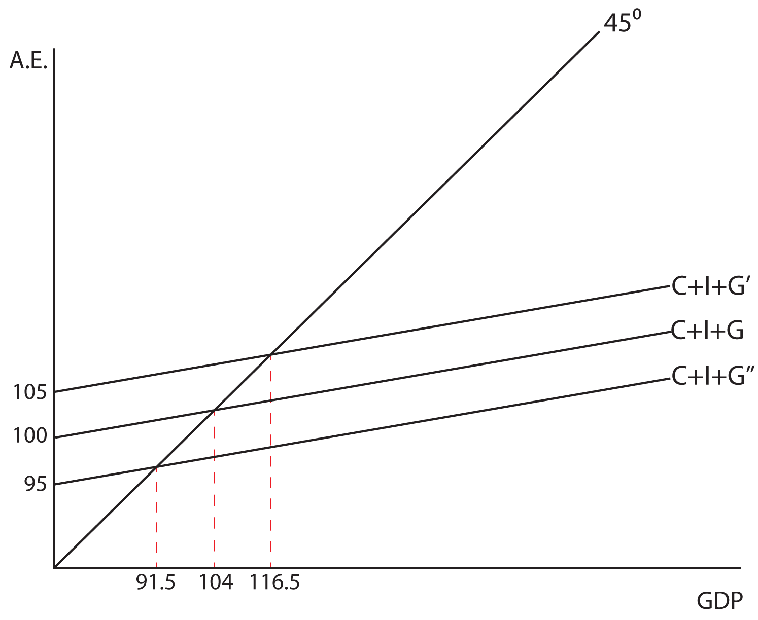
Retrieve About It: Calculating the Effect of the Counterbalanced Budget Multiplier

Demonstrate both graphically and algebraically the impact on GDP of increasing government spending and taxes by $5 billion dollars when the MPC is .9.

ALGEBRAIC Respond

The increase in G causes output to increase by $v billion x x = $150 billion.
The increases in taxes causes output to go down by $5 billion x nine = $45 billion.
The net result is that output increases by $5 billion. Shut (X)

GRAPHIC Reply

[insert Image 11.5 here]

The motility from C+I+G to C+I+G' is the increment in G of $v billion and the modify from C+I+M' to C'+I+G' is caused past the changes in taxes of $v. The overall change is an increase of $5 billion in the GDP. Close (X)

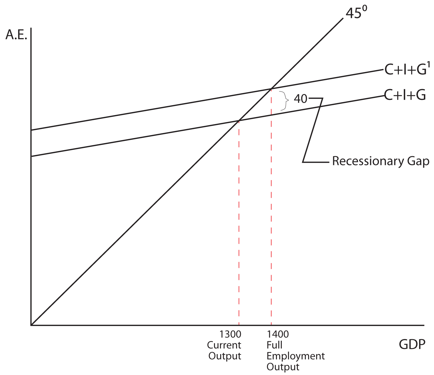
Section 03: The Recessionary and Inflationary Gaps

Permit's say that GDP = 1400 is the full employment output, or the equilibrium level we would like to obtain.  Also assume that the MPC is equal to .6. If the economy was actually producing 1300 and the government wanted to implement policies to increase output to 1400 they would need to increase government spending by 40. This additional forty in government spending is called the recessionary gap.

To change output in the economy from 1500 to 1400 you would have to reduce G by twoscore. In this case, the 40 in government spending is an inflationary gap.

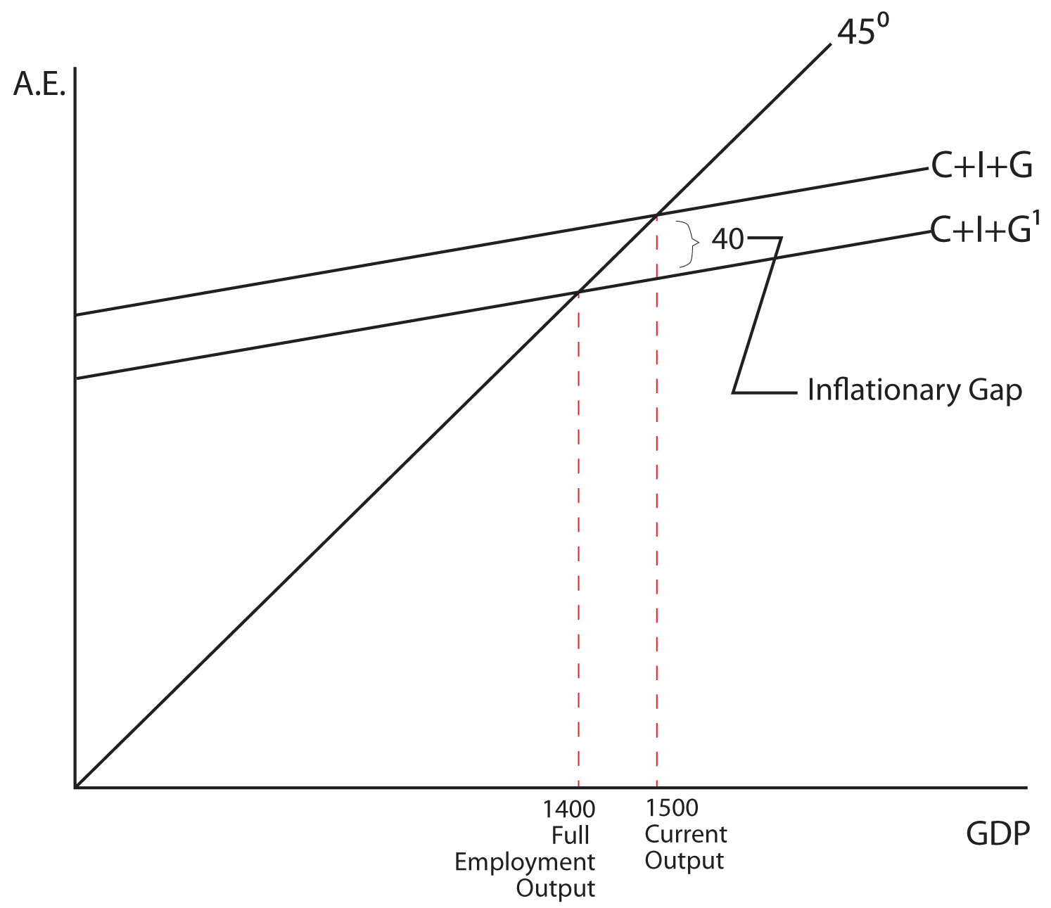
When 1000 is used to increase output, it is called anti-unemployment policy and when G is used to subtract output it is called anti-inflationary policy.

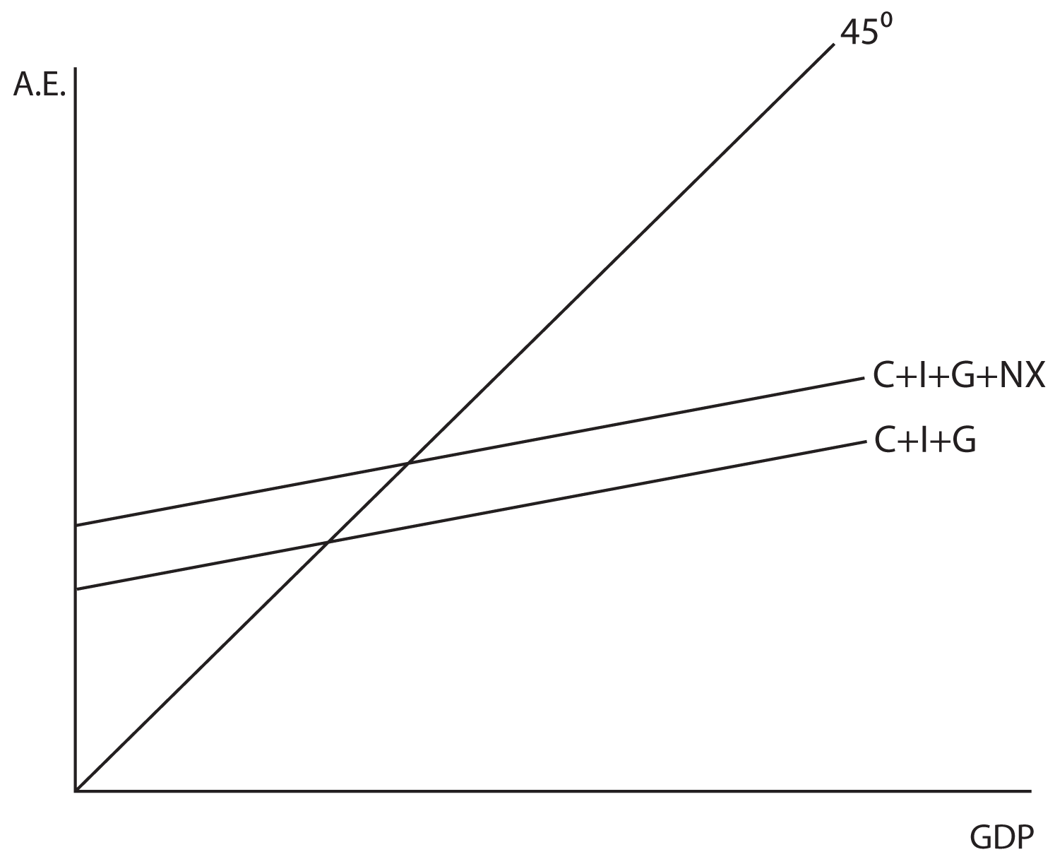
Cyberspace exports and Equilibrium Output

If we add international trade to our analysis and assume that net exports are independent of the level of GDP, then equilibrium GDP volition be determined by where the C+I+M+NX line intersects the 45 degree line in our standard model (come across the graphs below).

Changes in NX have a similar touch on on equilibrium Gdp as changes in investment or authorities spending take. For instance, if the MPC were equal to 0.5 and at that place were an increase in NX equal to $xv 1000000, the output would increase by $30 million. This is true because the multiplier would exist equal to ii.

Source: https://courses.byui.edu/econ_151/presentations/lesson_07.htm

Posted by: coxhalight.blogspot.com

Share this post